Advanced Usage Guide
Introduction
The Quick Start Guide provides a recommended basic usage for the Ill Conditioning Explainer. However, in a significant number of instances, large explanations that are difficult to interpret remain after executing the recommended workflow. This section will discuss how to effectively interpret the explainer output, including for larger explanations. In addition it will describe additional arguments to the explainer functions that can reduce the size of the explanations.
Interpreting the Explainer Output
The Quick Start Guide describes how to interpret the meaning of the rows or columns in the LP or MPS file generated by the explainer. However, extracting the specific cause of the ill conditioning from these files can be more challenging. This section provides some guidance on how to do so. Specifically, by making full use of the linear combination vector values and watching for common model structures that can cause ill conditioned basis matrices, even large explanations can often be used to effectively identify the source of the ill conditioning.
Regarding making full use of the linear combination vector values, recall from the Introduction section that the vector satisfies the condition \(||B^{T}y||_{\infty} \leq \epsilon\) and \(||y|| \gg \epsilon\). The explainer output lists the rows or columns ordered by largest absolute multiplier value. Small multiplier values can be ignored from consideration as long as the corresponding basis matrix row or column values are orders of magnitude larger than 1.0. In such cases, their contribution to the inner product \(B^{T}y\) is negligible. But if the row or column values are significantly larger, they still contribute significantly to the ill conditioning.
Regarding common model structures in ill conditioned models, three in particular have occurred both in the more than 15 years of Gurobi customer tickets and in the recent development of the Ill Conditioning Explainer. Searching for small subset of constraints or variables in a large explanation can often identify the source of ill conditioning without having to look at most of its contents.
Mixtures of large and small coefficients in matrix rows or columns. The definition of the condition number of a square matrix \(B\) is \(||B||\cdot||B^{-1}||\). Large ratios in B can easily result in large values in either \(||B||\) or \(||B^{-1}||\). In many cases such large ratios are unnecessary and can be avoided. For example, using more suitable units of measurements (e.g., counting in thousands of dollars rather than dollars) or reducing unnecessarily large values in big M constraints used to model fixed charges can often improve the large ratios without affecting the meaning of the model.
Imprecise rounding of matrix coefficient values. Rounded repeating decimals associated with fractions can turn truly parallel rows, which do not create issues with ill conditioning, into nearly parallel rows, which do. For models with fractional data with repeating decimal places, avoid imprecise rounding of these values, e.g., don’t calculate 1/3 or 5/7 to 10 decimal places instead of the full 16 decimal places that are available in the 64 bit doubles that Gurobi uses to input the problem data. Better yet, if the numerator and denominator of the fractions in a constraint are known when building the model, use the denominators to rescale the matrix row to have all integer data. For example, the constraint
1/3 x + 5/7 y <= 10can be multiplied 21 (the product of the denominators) to yield the all integer constraint7x + 15y <= 210, which will yield a more precise representation of the coefficients. Similarly, watch for matrix coefficients that are supposed to respresent the same value but have different levels of precision in different places. This happens surprisingly often, either because different parts of the model are created over time, or because values are calculated in mathematically equivalent ways that have slight differences when calculated under finite precision. For example, note the difference in the 16th decimal place of the following two mathematically equivalent values when calculated with Python:>>> import math >>> math.sqrt(2)/2 0.7071067811865476 >>> math.sin(math.radians(45)) 0.7071067811865475
Such slight differences can turn identical coefficients into slightly different ones, which in turn can transform truly parallel rows into almost parallel ones, thus creating ill conditioning. If the values are mathematically equivalent, they should be same to the lowest order bit in the LP or MIP, and care should be taken to ensure they are computed in the same way in the model generation process.
Long Sequences of Transfer Constraints. Transfer constraints multiply a variable by a number and assign the expression into a new variable. A long sequence of such constraints where each variable appears as output in one constraint and input in the next can implicitly create a large numeric value and a basis matrix with a high condition number. For example, consider
\[\begin{split}x_1 = 2x_2 \\ x_2 = 2x_3 \\ x_3 = 2x_4 \\ \vdots \\ x_{n-1} = 2x_n \\ x_j \geq 0, j=1,\cdots, n\end{split}\]These constraint have coefficients have neither imprecise rounding nor large ratios of coefficients, yet this structure can lead to an ill conditioned basis matrix. These constraints define a long sequence of transfers of variable activity levels, starting with \(x_n\) and ending with \(x_1\). Hence they imply the constraint \(x_1=2^{n-1}*x_n\), which does have a large coefficient ratio. Also, note that if any one of the variables \(x_j\) in the sequence of transfer constraints is positive, all of them will be, and they all will be basic. The associated square submatrix of the LP has the form
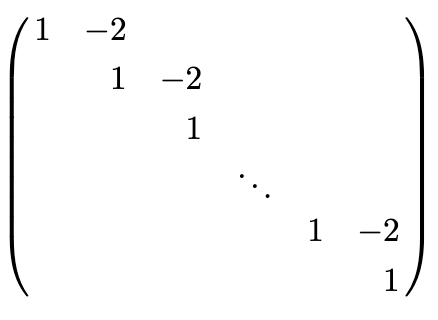
This submatrix has inverse of the form
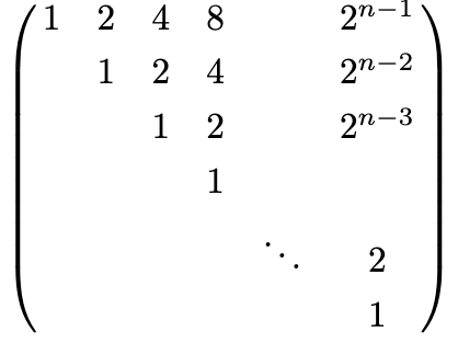
Given that the condition number of a square matrix \(B\) is \(||B||\cdot||B^{-1}||\), one can see that the submatrix of transfer constraints contributes \(2^{n-1}\) to the overall basis condition number. Hence it can be a source of ill conditioning for even modest values of \(n\).
Here is some sample ill conditioning explainer output of a long sequence of transfer constraints from a run on a subproblem of a publicly available model where the basis condition number was on the order of \(10^{31}\). Note that each variable appears in consecutive constraints, and that the coefficients in each constraint are the same. In this model the variables are free variables rather than being bounded below by 0.
(mult=1.267949192397407)e11923: 0.221528652 x33590 = 0(mult=-0.3397459621039425)e11803: 0.221528652 x32870 + 0.8267561847 x33590 = 0(mult=0.09103465616606164)e11683: 0.221528652 x32150 + 0.8267561847 x32870 = 0(mult=-0.02439266259987994)e11563: 0.221528652 x31430 + 0.8267561847 x32150 = 0(mult=0.006535994244062434)e11443: 0.221528652 x30710 + 0.8267561847 x31430 = 0(mult=-0.0017513143792112112)e11323: 0.221528652 x29990 + 0.8267561847 x30710 = 0(mult=0.00046926327354376596)e11203: 0.221528652 x29270 + 0.8267561847 x29990 = 0(mult=-0.00012573871516785733)e11083: 0.221528652 x28550 + 0.8267561847 x29270 = 0(mult=3.3691587182326145e-05)e10963: 0.221528652 x27830 + 0.8267561847 x28550 = 0(mult=-9.027633576094116e-06)e10843: 0.221528652 x27110 + 0.8267561847 x27830 = 0(mult=2.4189471259749366e-06)e10723: 0.221528652 x26390 + 0.8267561847 x27110 = 0(mult=-6.481549288572281e-07)e10603: 0.221528652 x25670 + 0.8267561847 x26390 = 0(mult=1.736725897357507e-07)e10483: 0.221528652 x24950 + 0.8267561847 x25670 = 0(mult=-4.6535430161276043e-08)e10363: 0.221528652 x24230 + 0.8267561847 x24950 = 0(mult=1.246913092958399e-08)e10243: 0.221528652 x23510 + 0.8267561847 x24230 = 0(mult=-3.341093562480668e-09)e10123: 0.221528652 x22790 + 0.8267561847 x23510 = 0(mult=8.952433217911677e-10)e10003: 0.221528652 x22070 + 0.8267561847 x22790 = 0(mult=-2.3987972507319496e-10)e9883: 0.221528652 x21350 + 0.8267561847 x22070 = 0(mult=6.427557860589595e-11)e9763: 0.221528652 x20630 + 0.8267561847 x21350 = 0(mult=-1.7222589378332707e-11)e9643: 0.221528652 x19910 + 0.8267561847 x20630 = 0(mult=4.614778914917941e-12)e9523: 0.221528652 x19190 + 0.8267561847 x19910 = 0(mult=-1.2365262833452548e-12)e9403: 0.221528652 x18470 + 0.8267561847 x19190 = 0(mult=3.3132621900063825e-13)e9283: 0.221528652 x17750 + 0.8267561847 x18470 = 0Finally, note that the ratio of the multipliers for consecutive constraints remains constant from start to finish, and is in fact the ratio of the two coefficients \(0.8267561847/0.221528652\). This example is similar to the first transfer constraint example, except that the variables are free instead of nonnegative, and the transfer coefficient is \(0.8267561847/0.221528652\) instead of 2.
Remedies for long sequences of transfer constraints are not as simple as for imprecise rounding or large ratios of coefficients in the basis matrix rows or columns. The model developer should assess the meaning of these constraints in the context of the whole model, and why the activities at the start of the sequence are implicitly being rescaled to much larger values at the end of the sequence.
The API Reference also includes two utility functions that can help with interpreting the explainer output. The matrix_bitmap function provides a bit map of the explanation’s matrix nonzero structure; this can be useful for detecting long sequences of transfer constraints, which will frequently exhibit a block diagonal matrix nonzero structure. The converttofractions function converts decimal values to their nearest rational representation; this can help with imprecise rounding, particularly when repeating decimals are involved.
For a more detailed discussion of common sources of ill conditioning in LPs and MILPs, see Section 4 of https://pubsonline.informs.org/doi/10.1287/educ.2014.0130.
Examples
Here are some examples from publicly available models that illustrate how to interpret explanations of nontrivial size. Each example illustrates one of the aforementioned three common model structures in ill conditioned models.
The LP relaxation of the MIPLIB model neos-1603965. This example illustrates mixtures of large aned small coefficients in matrix rows or columns. The original MIP can be downloaded from https://miplib.zib.de/instance_details_neos-1603965.html. The LP relaxation is available in the examples directory of this repository or by calling the Model.relax() function on the original MIP. The optimal basis condition number was on the order of \(10^{22}\) The row-based explanation file in the examples directory consists of 676 rows and 677 columns. As this is much smaller than the column-based explanation for this model, only this explanation will be discussed.
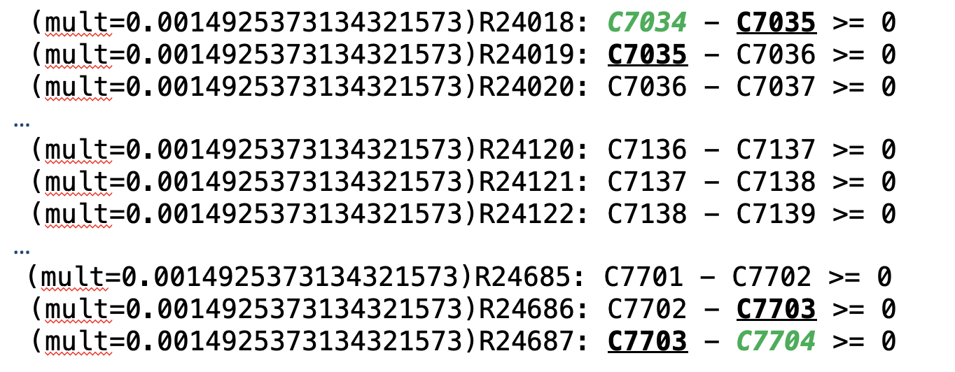
While an explanation of this size can be difficult to interpret in its entirety, one should first look for components of the explanation that involve one of the aforementioned three common model structures. Most of the constraints in the explanation have nothing in common with any of these characteristics, as they contain only +-1 coefficients and do not promote any growth in the variable values.
(mult=0.0014925373134321573)R24018: C7034 - C7035 >= 0(mult=0.0014925373134321573)R24019: C7035 - C7036 >= 0(mult=0.0014925373134321573)R24020: C7036 - C7037 >= 0…(mult=0.0014925373134321573)R24685: C7701 - C7702 >= 0(mult=0.0014925373134321573)R24686: C7702 - C7703 >= 0(mult=0.0014925373134321573)R24687: C7703 - C7704 >= 0Only 5 constraints differ from these, so it makes sense to focus on those.
(mult=1.4925373134321572e-13)R8030: C3030 - 1e+10 C7034 <= 0(mult=1.4925373134321572e-13)R12700: - C3700 + C3701 - 0.05 C7001+ 1e+10 C7704 <= 1e+10(mult=1.4925373134321572e-13)R28684: C3700 = 6630(mult=-1.4925373134321572e-13)R28685: - C1701 + C3701 = 7065(mult=-1.4179104477605494e-13)R28014: C0030 + C3030 = 7165One sees large coefficient ratios in rows R8030 and R12700. Based just on these 5 constraints the explanation suggests that the 1e+10 coefficients are probably big M values that could be reduced without compromising the meaning of the constraints, or replaced with the more numerically stable indicator constraints that Gurobi offers.
Reducing or eliminating the big M values of 1e+10 is probably enough to resolve the ill conditioning, so the remaning 671 constraints in the explanation could be ignored. However, let’s try to understand the explanation in its entirety to help prepare for other explanations where ignoring significant parts is not an option.
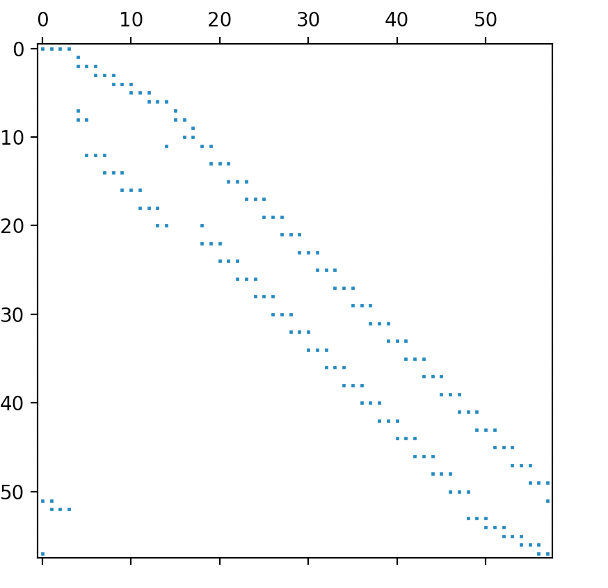
Running the matrix_bitmap program on the full explanation sheds light on how the remaining 671 constraints contribute to the high optimal basis condition number. The resulting bitmap reveals a nonzero structure of bidiagonal elements except for a small block at the bottom right.
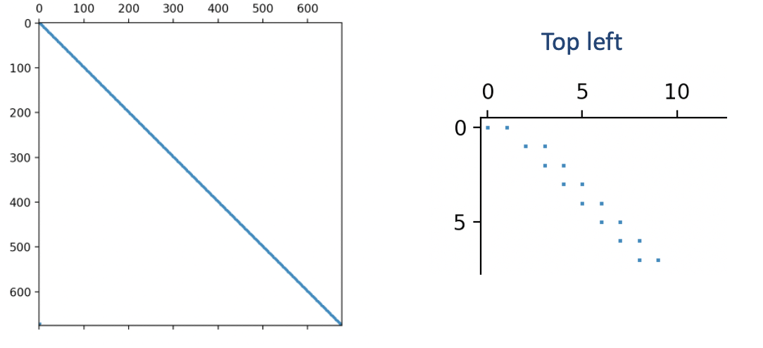
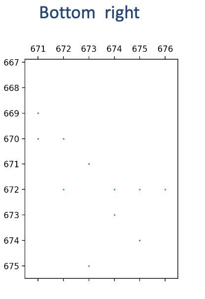
The bitmap indicates that consecutive bidiagonal constraints have a variable in common. This is indeed true, and a closer look reveals that adding these constraints results in cancellation of the common variables.
Indeed, after adding all these constraints, only variables C7034 and C7704 remain. The complete explanation now reduces down to this combined constraint along with the 5 remaining constraints that were excluded from the summation process.
Combined: C7034 - C7704 >= 0R8030: C3030 - 1e+10 C7034 <= 0R12700: - C3700 + C3701 - 0.05 C7001 + 1e+10 C7704 <= 1e+10R28684: C3700 = 6630R28685: - C1701 + C3701 = 7065R28014: C0030 + C3030 = 7165From just these constraints one can construct a nonzero vector
\(y=(1, 10^{-10}, 10^{-10}, 10^{-10}, -10^{-10}, -10^{-10})\)
that satisfies the condition of a certificate of ill conditioning, namely \(||B^{T}y||_{\infty} \leq \epsilon\) and \(||y|| \gg \epsilon\). One can extend the certificate to the other 671 constraints involving bidiagonal constraints by setting each y value to 1 as well, i.e., for the full explanation the vector with 676 components
\(y=(1, 1, \cdots, 1, 10^{-10}, 10^{-10}, 10^{-10}, -10^{-10}, -10^{-10})\)
satisfies the certificate of ill conditioning criterion in the same way, namely
\(y^{T}Bx = 10^{-10} C0030 + 10^{-10} C1701 - 5*10^{-12} C7001\)
has only small coefficients.
The LP relaxation of the MIPLIB model ns2122603. This example illustrates a combination of imprecise rounding and mixtures of large and small coefficients. The original model can be downloaded from the unstable set at https://miplib2010.zib.de/miplib2010-unstable.php. The LP relaxation is available in the examples directory of this repository or by calling the Model.relax() function on the original MIP. The optimal basis condition number was on the order of \(10^{10}\). The row-based explanation consists of 241 constraints and 241 variables, while the column based explanation consists of 187 constraints and 187 variables. Both reside in the examples directory of the repository. Given the similar sizes, the discussion here will consider the row-based explanation.
An interpretation of all 241 constraints in the row-based explanation, while possible, is not really needed. As with the previous example, searching for the three common model structures. will suffice. Using the converttofractions function if needed, one sees numerous constraints with the fraction 1/24 represented with only 7 decimal places and some rounding of the repeating decimal representation.
(mult=0.011788497081319169)R2209: C6379 - C6380 - 0.0416667 C14243 >= 0(mult=0.011732361380931935)R2208: C6378 - C6379 - 0.0416667 C14242 >= 0(mult=0.011676492993403688)R2207: C6377 - C6378 - 0.0416667 C14241 >= 0Coefficients like these could be represented exactly as, for example,
R2209better: 24 C6379 - 24 C6380 - C14243 >= 0Additionally, other constraints have coefficients with rounding errors in the 6th and 8th decimal places.
(mult=-5.640429225511564e-05)R5989: C6380 - 8.750007 C14244 <= 0.02083335(mult=-5.613570038723414e-05)R5988: C6379 - 8.750007 C14243 <= 0.02083335These coefficients are clearly intended to be 35/4 and 1/48 respectively. Using those exact coefficients and multiplying by the least common denominator of 48 yields, for example,
R5989better: 48 C6380 - 420 C14244 <= 1Additional constraints in the explanation indicate unnecessarily large big M coefficents.
(mult=4.144857381208667e-12)R13507: 1e+08 C14195 - 1e+08 C12855 - 0.0416667 C11595 >= -1e+08These big M coefficients can either be reduced without compromising the meaning of the model or replaced with indicator constraints.
An LP subproblem associated with the open MINLPLIB model topopt-cantilever_60x40_50. This example was already discussed in the second transfer constraint example and will not be repeated here. However, the model and row based explanation are available in the examples directory of the repository. The easiest way to reproduce the basis with high condition number is to read in the cantilever_sublp.bas file that is included in the examples directory. Or, run the LP with presolve off.
The irish-electricity LP model from the Mittelmann benchmark set. This example illustrates a more elaborate sequence of transfer constraints. The model can be downloadeded from https://plato.asu.edu/ftp/lptestset/irish-electricity.mps.bz2 and is also available in the examples directory of this repository. It is the LP relaxation of the MIPLIB 2017 model of the same name that involves a unit commitment model for electrical power generation. The optimal basis condition number was on the order of \(10^{38}\). The row-based explanation size consists of 57 constraints and 58 variables, while the column-based explanation consists of 4698 constraints and 4431 variables. Given it’s much smaller size, the discussion here will focus on the row-based explanation.
Examination of the bit map generated by the matrix_bitmap function indicates a nonzero pattern consistent with a long sequence of transfer constraints.
However, this is more complicated than either of the previous examples of sequences of transfer constraints, both of which had a simple bidiagonal nonzero pattern. The row based explanation appears to involve variables and constraints associated with activities for a single power source and multiple time periods. However, the explanation sorts the constraints in descending order by absolute multiplier value, and the connection between consecutive time periods is not immediately clear.
(mult=1.473670931920553)MinDownInit_24: v_24_13 = 0(mult=-0.301174019398261)Link_u_v_24_14: v_24_13 + u_24_13 - v_24_14 >= 0(mult=-0.11503823888171555)Link_u_v_24_15: v_24_14 + u_24_14 - v_24_15 >= 0(mult=-0.04394069724688566)Link_u_v_24_16: v_24_15 + u_24_15 - v_24_16 >= 0(mult=-0.01678385285894142)Link_u_v_24_17: v_24_16 + u_24_16 - v_24_17 >= 0(mult=-0.006410861329938599)Link_u_v_24_18: v_24_17 + u_24_17 - v_24_18 >= 0…(mult=0.001128095639494215)RampUpSlow_P_24_14: - 165 u_24_13 - 165 v_24_14 + 165 u_24_14 <= 0(mult=-0.0009353320626839298)Link_u_v_24_20: v_24_19 + u_24_19 - v_24_20 >= 0(mult=0.0004308941917262418)RampUpSlow_P_24_15: - 165 u_24_14 - 165 v_24_15 + 165 u_24_15 <= 0(mult=-0.00035726505717771395)Link_u_v_24_21: v_24_20 + u_24_20 - v_24_21 >= 0(mult=0.00016458693568451054)RampUpSlow_P_24_16: - 165 u_24_15 - 165 v_24_16 + 165 u_24_16 <= 0Examination of the primal and dual variables associated with the ill conditioned basis can shed light on how the transfer constraints interact. The definition of the condition number of a square matrix \(B\) is \(||B||\cdot||B^{-1}||\). Given that the problem statistics for this LP (which can be obtained by calling Gurobi’s Model.printStats() method) indicate that the original constraint matrix has coefficients of very modest orders of magnitude, \(||B^{-1}||\) must contain some large coefficients. Given that the primal and dual variables of the LP involve linear combinations of columns and rows of \(||B^{-1}||\) respectively, large primal or dual values may shed light on constraints involved in the ill conditioning and how they are sequenced. For the basis in question, there are no large primal values. However, numerous large dual values exist, including for the power sources and time periods in the explanation. The following image reveals dual values for the relevant power source that increase as the time period decreases. Underlined constraints appear in the row-based explanation.

This suggests that the Link and RampUpSlow constraints for consecutive time periods are related, as the dual variables steadily increase as the time period decreases. Therefore, reordering the Link and RampUpSlow constraints in descending order by time period may be a useful reordering of the explanation that will facilitate interpretation. In other words, reorder the constraints in the explanation as follows and start with the constraints with the largest time period.
(mult=-0.11503823888171555)Link_u_v_24_15: v_24_14 + u_24_14 - v_24_15 >= 0(mult=0.0004308941917262418)RampUpSlow_P_24_15: - 165 u_24_14 - 165 v_24_15 + 165 u_24_15 <= 0(mult=-0.04394069724688566)Link_u_v_24_16: v_24_15 + u_24_15 - v_24_16 >= 0(mult=0.00016458693568451054)RampUpSlow_P_24_16: - 165 u_24_15 - 165 v_24_16 + 165 u_24_16 <= 0(mult=-0.01678385285894142)Link_u_v_24_17: v_24_16 + u_24_16 - v_24_17 >= 0…(mult=2.738820795076575e-13)RampUpSlow_P_24_37: - 165 u_24_36 - 165 v_24_37 + 165 u_24_37 <= 0(mult=-2.824408944922718e-11)Link_u_v_24_38: v_24_37 + u_24_37 - v_24_38 >= 0(mult=1.0270577981537156e-13)RampUpSlow_P_24_38: - 165 u_24_37 - 165 v_24_38 + 165 u_24_38 <= 0(mult=-1.1297635779690872e-11)Link_u_v_24_39: v_24_38 + u_24_38 - v_24_39 >= 0Consider the last two constraints Link_u_v_24_39 and RampUpSlow_P_24_38. Both of them intersect the variable u_24_38, so one can multiply Link_u_v_24_39 by -165 and add it to RampUpSlow_P_24_38 to eliminate u_24_38 and v_24_38. Then consider the resulting combined constraint with Link_u_v_24_38, the next constraint in the sequence.
combinedcon0: - 165 u_24_37 - 330 v_24_38 + 165 v_24_39 <= 0Link_u_v_24_38: v_24_37 + u_24_37 - v_24_38 >= 0Both of them intersect the variable v24_38, so one can multiply Link_u_v_24_38 by -330 and add it to the combined constraint to obtain another combined constraint. Then consider this new constraint with RampUpSlow_P_24_37.
combinedcon1: - 495 u_24_37 + -330 v24_37 + 165 v_24_39 <= 0RampUpSlow_P_24_37: - 165 u_24_36 - 165 v_24_37 + 165 u_24_37 <= 0These two constraints both intersect u_24_37, so one can multiply RampUpSlow_P_24_37 by 3 to obtain another combined constraint.
combinedcon2: -825 v24_37 -495 u_24_36 + 165 v_24_39 <= 0Note that the growth in the combined constraint is now starting to accelerate. One can continue this process of multiplying the next explanation constraint by a value that results in a combined constraint with only 3 nonzeros. Here is a summary of some additional operations of this type. Note that accelerating growth of the largest coefficient in the combined constraint.
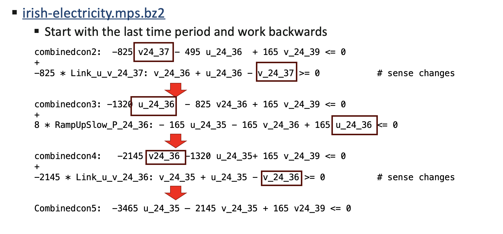
In each of the combined constraints, the largest coefficient is a multiple of -165 One can assess the growth rate by looking at the sequence of integer multiples of -165 in the series of combined constraints.
This is the Fibonacci sequence, for which Binet’s formula gives value of the n-th Fibonacci number.
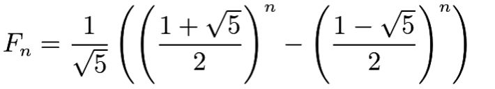
This pattern continues throughout the explanation and illustrates the the growth rate of the largest coefficient in the combined constraint occurs at an exponential rate. The pivoting operations described here mimic those used to obtain the inverse of the basis matrix, thus explaining the source of the ill conditioning.
The question remains of how to remedy the cause of ill conditioning. In the previous example models, the ill conditioning could be reduced or avoided by addressing unnecessarily imprecise rounding of important coeffients, or reducing unnecessarily large coefficient ratios in the constraint matrix rows or columns. No such simple remedy is available. The model is publicly available, and the LP is the relaxation of the MIPLIB 2017 model of the same name, which is a Unit Commitment model. Examination of the solution and basis file associated with this optimal but ill conditioned basis that the u and v variables in the explanation are all basic, but at their lower bound of 0. Therefore, the ill conditioning was relatively harmless for the model in its current state; it did not adversely affect primal or dual solution quality. A paper at https://inria.hal.science/hal-01665611/file/UC_CMBA.pdf that describes the model indicates that these constraints involve available power and suggests that if all available power was used over an extremely large number of time periods, huge power production costs would result. However, apparently such a solution will not be used in practice. However, a small change to the model that would enable the u and v variables to take on positive values could yield drastically different results.
Additional Function Arguments
The Quick Start Guide describes the most common usage of the explainer functions kappa_explain and angle_explain. This section considers additional function arguments that can help reduce the size of the explanation, potentially making it easier to interpret. A complete list of function arguments appears in the API Reference section.
The kappa_explain() method
The kappa_explain method provides a row or column based explanation of the cause of ill conditioning in a basis matrix. It has several arguments designed to reduce the size of the explanation.
The expltype parameter instructs the explainer to provide a row or column based explanation. As discussed in the Quick Start Guide, one of these two explanations may be smaller and easier to interpret than the other. Set this parameter to “ROWS” or “COLS” for a row or column based explanation respectively. In general if the first explanation you try among these two seems too large or difficult to interpret, try the other one.
The smalltol parameter specifies the tolerance used with the certificate of infeasibility to filter out rows or columns of the basis matrix in the explanation. Recall from the Introduction section that the certificate of infeasibility vector y satisfies \(||B^{T}y||_{\infty} \leq \epsilon\) and \(||y|| \gg \epsilon\). Elements of y that are zero identify basis matrix rows or columns that can be removed from the explanation. However, in numerous explanations, rows or columns with small multipliers contribute little insight to the explanation and can be ignored. The smalltol parameter is optional, and by default the explainer will use a base value of \(10^{-13}\), but also consider each row or column norm as well as the machine precision. Specifying a non default value other than \(10^{-13}\) replaces the default setting with the alternate value to be used in the row or column filtering process. Note that the explainer output file lists the rows or columns ordered in descending order starting with the absolute multiplier value, so one can visually filter the small multipliers as well. Keep in mind that equal multipliers does not imply equal contribution to the ill conditioning. A small multiplier associated with a row or column with all (absolute) coefficient values at most 1 contributes significantly less then the same multiplier associated with a row or column with coefficient values on the order of \(10^{8}\)
The method parameter enables alternate formulations of the internal model that computes the certificate of ill conditioning. These options currently involve regularization methods of the objective that try to reduce the size of the explanation. The default setting performs no regularization. The “ANGLES” option invokes the angle_explain method, which will be discussed subsequently. When invoked from kappa_explain with method=”ANGLES”, a single pair of almost parallel rows or columns will be returned, if it exists. Setting method=”LASSO” invokes the Lasso method, which involves adding a regularization term to the objective consisting of the sum of absolute values of the certificate variables. Setting method=”RLS” uses regularized least squares instead, which instead uses the sum of squares of the certificate variables.
The submatrix parameter performs postprocessing of the computed explanation to try to reduce the size. The default setting is False; set it to True to enable this feature. Initial tests with this parameter show reductions in explanation size of 20-50 percent. Unfortunately, however, this level of reduction may have limited value on large explanations of hundreds or thousands of rows or columns, as the explanation remains quite large after this postprocessing is performed.
The angle_explain() method
The angle_explain method looks for near parallel pairs of basis matrix rows or columns. It does not solve a subproblem. The explanations it finds, if any exist, are always easy to interpret. But for many ill conditioned basis matrices no near parallel pairs exist, and the routine provides no information (other than the fact that any explanation has at least 3 rows or columns). It is simpler to use, and the only required argument is the LP model. Two other parameters provide some additional control.
The howmany parameter specifies the number of near parallel rows and columns to search for. If not specified, this defaults to 1. Specify a positive integer for a particular number of pairs. Specify an integer <= 0 to request all pairs. The routine searches the rows first, then the columns. Requesting more pairs can increase the run time of the routine.
The partol parameter specifies the tolerance below which two row os column vectors are considered almost parallel. It defaults to \(10^{-6}\). It is used as a relative tolerance when comparing the inner product of two vectors with the product of their L1 norms.